 BTR Enerji · Solar Tracker
GCR Optimization: Should Tracker Row Spacing Follow LCOE or NPV?
Ground coverage ratio (GCR) sets how densely tracker rows are packed. We scanned the same site in Konya, Seville and Bavaria from GCR 0.20 to 0.50 in our simulator. The result is clear: the lowest LCOE came at the sparsest layout (GCR 0.20) at every site, while the highest NPV came at the densest layout (GCR 0.50) when grid capacity was unlimited. Fix the grid capacity and the picture changes: the optimum falls to GCR 0.32–0.35.
The short answer
When land is limited, choosing GCR on LCOE alone is misleading: LCOE rewards the sparse layout in which each module is least shaded, and leaves part of the capacity the land could hold unused. An investor's real yardstick is total value (NPV). But NPV does not rise forever either: if the grid connection capacity is fixed, beyond a certain density every added module is clipped more and more and NPV starts to fall. The right GCR comes from reading LCOE and NPV together and accounting for grid capacity, land cost and backtracking limits.
What is GCR and why does it matter?
GCR (ground coverage ratio) is module width divided by row pitch. GCR 0.30 means a row pitch of about 8 m for a 2.4 m wide tracker row. A higher GCR fits more modules on the same land, but rows shade each other earlier in the morning and evening; the tracker backtracks earlier to avoid shading and output per module falls.
How did we calculate it?
We used our simulator's GCR optimization tool: for each GCR the layout, energy, bill of materials and financial model were recalculated from scratch. Common assumptions:
- 10 hectares of flat land, north-south single-row (1P) tracker with backtracking, 710 W bifacial modules;
- PVGIS typical meteorological year; losses (temperature, soiling, cabling, inverter clipping, transformer) identical in every scenario;
- The simulator's default electricity price (0.09 USD/kWh) and a fixed installed cost per MWp; land cost not included.
Because absolute prices vary by project, we show LCOE and NPV as an index with GCR 0.30 = 100.
GCR scan in Konya: LCOE and NPV move in opposite directions
| GCR | Capacity (MWp) | Specific yield (kWh/kWp·yr) | LCOE index | NPV index, no grid cap | NPV index, grid capped at 4.8 MW |
|---|---|---|---|---|---|
| 0.20 | 3.77 | 2,323 | 96 | 70 | 72 |
| 0.25 | 4.73 | 2,282 | 98 | 86 | 88 |
| 0.30 | 5.66 | 2,244 | 100 | 100 | 100 |
| 0.32 | 6.04 | 2,238 | 100 | 106 | 101 |
| 0.35 | 6.61 | 2,215 | 101 | 114 | 100 |
| 0.40 | 7.54 | 2,174 | 103 | 127 | 96 |
| 0.45 | 8.50 | 2,131 | 105 | 138 | 89 |
| 0.50 | 9.45 | 2,092 | 107 | 149 | 81 |
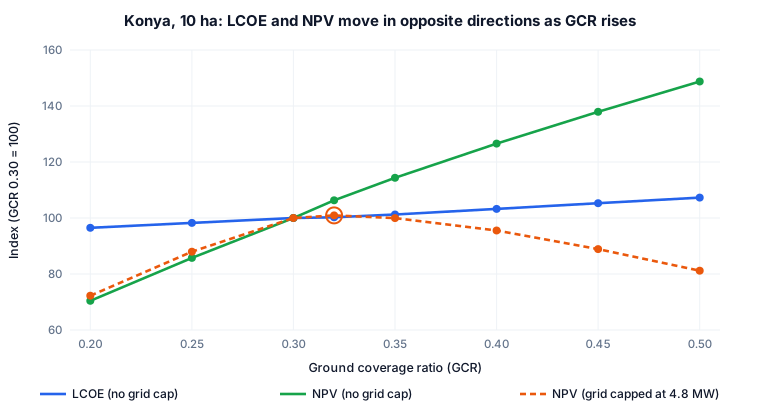
Going from GCR 0.20 to 0.50 raises capacity from 3.77 MWp to 9.45 MWp, while specific yield drops from 2,323 to 2,092 kWh/kWp, or 10.0%. So LCOE climbs steadily, while NPV keeps rising because every added megawatt is still profitable.
Why does LCOE alone point the wrong way?
LCOE is an average: the mean cost of every kWh the plant produces. Investment decisions are made at the margin: if the cost of the energy added by densifying is below its sale or self-consumption value, NPV rises. In Konya the energy added between GCR 0.20 and 0.25 costs 106% of the GCR 0.30 LCOE, and between 0.45 and 0.50 it costs 129%. That energy pulls the average up at every step, yet it is still worth more than it costs, so NPV grows. Minimising LCOE effectively means "leave part of the land empty".
Pick your location and draw your land on the map. Get hourly-weather-based yield, a tracker vs fixed-tilt comparison, a bill of materials and the payback period, free of charge.
Free Solar Tracker Simulation
Where is the optimum when grid capacity is fixed?
In real projects grid connection capacity is usually set in advance. To model this we fixed it at the AC capacity of the GCR 0.30 layout, 4.8 MW. Now the DC capacity added by densifying is clipped more and more around midday. In Konya the energy added between GCR 0.35 and 0.40 costs 4.6 times the GCR 0.30 LCOE and NPV falls; at GCR 0.50 the NPV index drops to 81.
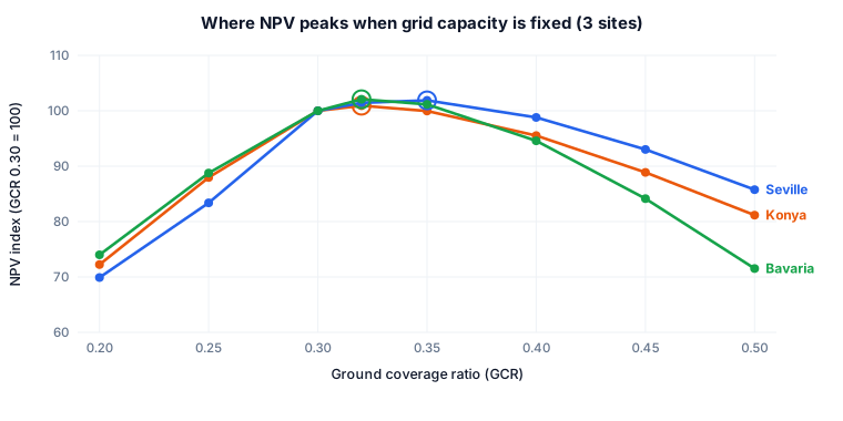
At all three sites NPV peaks between GCR 0.32 and 0.35: 0.32 in Konya and Bavaria, 0.35 in Seville. The peak is flat; the NPV difference between 0.30 and 0.35 is only a few points. Within that band site factors such as maintenance roads, pile layout and terrain slope matter as much as the financials.
How to choose GCR in design
- Identify the binding constraint first: is it land, grid capacity or budget? With limited land and flexible grid capacity, dense layouts win; with fixed grid capacity, a moderate GCR does.
- Include land cost: land is free in our calculation. Adding lease or purchase cost strengthens the case for denser layouts.
- Think about DC/AC ratio at the same time: with fixed grid capacity, raising GCR is really raising the DC/AC ratio; track clipping losses separately.
- Mind backtracking: at high GCR the tracker backtracks longer in the morning and evening, and bifacial rear-side gain also falls (see bifacial modules and albedo).

Method and limits
- Model: our pvlib-based simulator (backtracking, bifacial irradiance, temperature, soiling, cabling, inverter clipping, transformer); finance: 25-year discounted cash flow including inverter replacement in year 13.
- Simplifications: land cost and density-dependent cabling cost differences are limited; inverter size steps cause small jumps at some intermediate points.
- These are simulation results, not measurements. You can run the same scan for your own site with your layout, prices and grid capacity; for uncertainty see P50 and P90 explained.
Related: Solar tracker vs fixed-tilt · Solar tracker energy gain at 25 sites · Terrain-aware backtracking.
Frequently asked questions
What is the ideal GCR for a single-axis tracker?
There is no single right value. In our simulations with fixed grid capacity, NPV peaked between GCR 0.32 and 0.35 at three sites; with unlimited grid capacity and limited land, denser layouts gave higher NPV.
Should GCR be optimised for LCOE or NPV?
For limited land, NPV. LCOE is the average cost per kWh and always picks the sparsest layout; NPV measures the total value the land delivers. LCOE is still useful for comparison against the energy price.
How much does tracker yield fall as GCR rises?
In Konya, raising GCR from 0.20 to 0.50 cut specific yield from 2,323 to 2,092 kWh/kWp (10.0%), while capacity on the same land rose about 2.5 times.
Why does grid capacity change the GCR choice?
With fixed grid capacity, raising GCR raises the DC/AC ratio, so output from added modules is clipped more and more at midday. Beyond a point the added investment no longer pays back and NPV falls.
We deliver the whole project: feasibility, engineering, procurement, installation and grid connection, in Türkiye and abroad. Simulate your site for free first, then let our team prepare a tailored quote.
Start the Simulation and Get a Quote
The ratios on this page are typical industry ranges and are not binding; exact values are determined by a site-specific analysis.